Every travel demand study starts with a simple question: how many people leave each place, and where do they go? The Origin-Destination (O/D) matrix is the table that holds the answer. In this post I explain how it is built and how to read its rows, columns and diagonal. I also show why the same data is now usually stored in a different format, the stacked one.
Before the matrix: zones and centroids
To count trips, you first divide the territory into Traffic Analysis Zones (TAZ). Each zone is an area treated as a single unit. In the model, it is represented by a single point, the centroid, where trips “leave” from and “arrive” at.
In Brazil, the practical reference is the São Paulo Metro Origin-Destination Survey. In any survey, the choice of zones is not neutral: whatever stays inside a zone disappears from the analysis between zones.
What the O/D matrix is
Formally, the O/D matrix is a square two-way table, with as many rows and columns as there are zones (n x n). Each cell T_ij holds the volume of trips that start in origin zone i and end in destination zone j. This volume refers to a defined period (IPEA). The period matters: a morning peak matrix and a full-day matrix describe different phenomena.
Classic demand modeling has four steps: trip generation, distribution, mode choice and network assignment. The O/D matrix is the output of the second step, when the trips generated in each zone are distributed among the possible destinations (MIT, lecture on the four-step model).
How to read it: rows, columns and diagonal
The reading convention is stable: rows are origins, columns are destinations. With three zones, A, B and C, the table looks like this:
| Origin \ Destination | A | B | C | Total produced |
|---|---|---|---|---|
| A | T_AA |
T_AB |
T_AC |
O_A |
| B | T_BA |
T_BB |
T_BC |
O_B |
| C | T_CA |
T_CB |
T_CC |
O_C |
| Total attracted | D_A |
D_B |
D_C |
T |
The main diagonal (T_AA, T_BB, T_CC, where origin and destination are the same) records only intrazonal trips: trips that start and end inside the same zone. The other cells hold interzonal trips. The IPEA report draws attention to the weight of these trips held in the diagonal. That weight depends on how the zoning is drawn.
Marginal totals reveal the hubs
Summing a row gives the total trips produced by the origin zone: O_i = Σ_j T_ij. Summing a column gives the total trips attracted by the destination zone: D_j = Σ_i T_ij. The sum of all cells is the total number of trips in the study area, and it is the same whether you add up rows or columns (MIT; TU Delft).
In practice, these totals answer a common planning question: which zones generate many trips and which attract many. Generally, the generators are residential neighborhoods, and the attractors are employment and service centers.
Production-Attraction is not Origin-Destination
One distinction confuses a lot of people. The Production-Attraction (PA) matrix organizes trips around the traveler’s home, regardless of the direction of travel. So the trip to work and the trip back home count for the same producing zone. The O/D matrix, on the other hand, is directional and tied to a time window.
That is why the morning peak O/D matrix is asymmetric, with a strong flow from the outskirts to the center. The afternoon peak matrix shows the reverse movement. Anyone who uses a PA matrix as if it were O/D loses that direction.
Fitting the matrix to observed totals
A matrix that comes from a sample or a model rarely matches real traffic or passenger counts. To reconcile the two, analysts use biproportional balancing, known as Iterative Proportional Fitting (IPF) or the Furness and Fratar method. It rescales rows and columns alternately until the matrix’s marginal totals converge to the observed volumes (MIT, lecture on O/D inference; IPEA).
Another family of methods is the doubly constrained gravity model. It distributes trips according to impedance, that is, the cost of going from one zone to another (time, distance or generalized cost). At the same time, it respects the production and attraction totals (TU Delft). The same TU Delft notes also cover methods that update the matrix using growth factors.
Where the data comes from
Decennial household surveys, such as the São Paulo Metro survey, remain the ground truth used to statistically expand the sample. They are increasingly combined with electronic fare collection microdata (smart cards), which record every boarding. A master’s thesis from the Polytechnic School of the University of São Paulo (USP) shows how to build public transport O/D matrices from these records by chaining each card’s trips.
New sources bring their own caveats. A study using cellular network data in Norrköping, Sweden compared demand inferred from mobile phones with the municipality’s demand model. Agreement was weak at the original zoning. It became significant when trips were aggregated into fewer zones. The authors also observed systematic differences between the matrices depending on the method used to extract the trips.
The stacked format
The n x n table is the classic way to display the matrix, but it is not the most practical way to store it. In the stacked format (also called long, or tidy), each row of the table is an origin-destination pair. The flow and other attributes go in explicit columns:
| origin | destination | trips | mode | period |
|---|---|---|---|---|
| A | B | T_AB |
bus | AM peak |
| A | C | T_AC |
bus | AM peak |
| B | A | T_BA |
car | AM peak |
The Federal Highway Administration (FHWA) report documents this conversion between tabular survey data and the matrix files used by software such as TransCAD. The stacked format fits directly into relational databases and data science libraries such as Pandas, GeoPandas and dplyr. It also lets you drop pairs with no trips, instead of storing a cell with a zero.
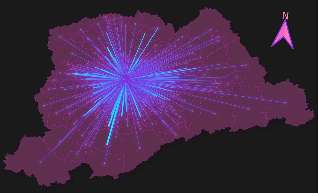
On top of that, the stacked format is the natural input for generating desire lines in QGIS. Each row of the table becomes a segment connecting two centroids, with thickness proportional to the flow.
The shape of the matrix itself is under discussion in research. An article in IEEE Transactions on Intelligent Transportation Systems argues that the traditional O/D matrix can lose geographic information. As an alternative, the authors propose a different structure, the O/D tensor, to feed forecasting models.
One limitation of this post: the material I gathered does not include measurements of the memory or processing cost of each format. So I do not compare performance here, only how the data is organized.
Takeaways
When you open an O/D matrix, check four things:
- the zoning used;
- the period it covers;
- whether the table is PA or O/D;
- whether the marginal totals were fitted to observed counts.
If your next step is analysis in Python, in R or in a geographic information system, store the data in the stacked format. Save the n x n table for presentation.
From matrix to desire lines: the Desire Lines plugin
That last step is why I built Desire Lines, a plugin that creates desire lines from an O/D matrix. It works with both versions discussed in this post: the n x n table and the stacked format. That way, the matrix can go in whichever format it reached you, and each origin-destination pair becomes a line connecting two centroids.