Logis, my new QGIS plugin, has been approved in the official plugin repository as version 0.1.8, flagged experimental. It groups logistics tools into three modules, and the reason for this post is the urban waste collection one: divide the municipality into sectors, trace the truck’s route street by street and measure how much of the trip is productive.
Almost nothing free for urban logistics
Anyone who has to plan collection, delivery or facility location in Brazil has two options today. The first is proprietary routing software, which solves the problem and charges an annual licence well outside the budget of most small municipalities. The second is research code, published as a script or a notebook, which works but assumes a Python environment already set up, dependencies installed and someone willing to deal with a traceback.
The professional working in QGIS, the standard tool in city halls and in small consultancies, is left without a way in. Logis exists to fill that gap: its 25 algorithms show up in the Processing Toolbox like any other QGIS process, with an input layer, parameters and an output layer.
Waste collection is arc routing
Most of the routing tools available solve a point visiting problem: there is a set of stops with known coordinates, and the question is the order in which to visit them. That is the travelling salesman formulation and its capacitated variants, and it describes a parcel delivery operation well.
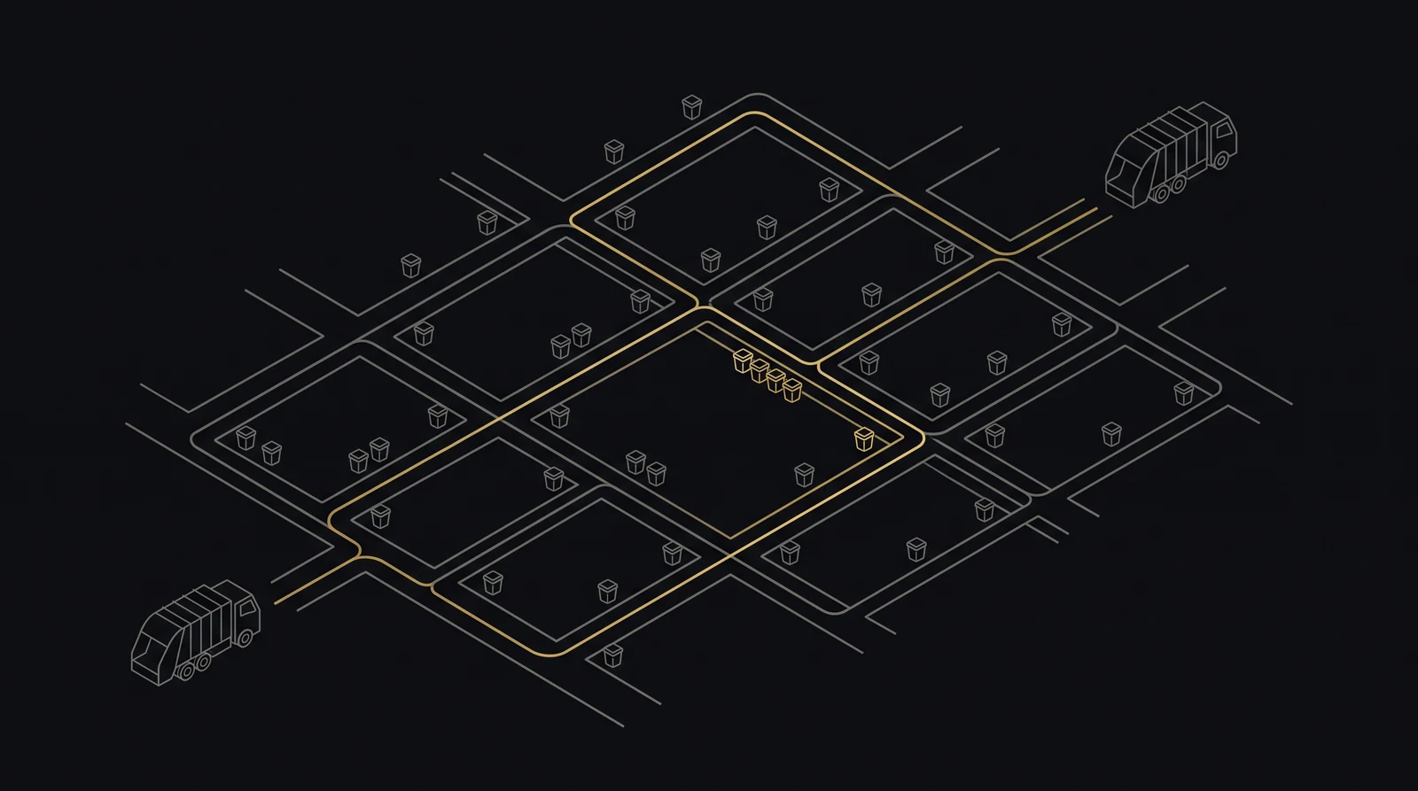
Household collection does not work that way. The truck does not visit points, it covers the length of the street: what has to be served is the whole street, and both sides of it when there are containers on both sides. Modelling every property as a stop produces a problem too large to solve in useful time and still describes the real operation poorly, since the vehicle crawls along while the collectors follow on foot. The right formulation is arc routing, which has three classic cases, all of them in the plugin:
- CPP (Chinese Postman Problem): cover every street in the sector at least once, returning to the starting point, with the shortest total distance. It fits when the whole network in the sector receives collection.
- RPP (Rural Postman Problem): only a subset of the streets needs collection, and the rest serve as passage. This is the most common case, because streets with no households, highway stretches and streets served by another sector generate no waste.
- CARP (Capacitated Arc Routing Problem): the truck fills up before finishing the sector and has to unload. The route stops being a single circuit and becomes a sequence of trips, each one limited by the vehicle’s capacity, with a leg out to the disposal site and back.
Zone it, size the fleet, measure what is left over
Tracing the route is the middle of the work, not the beginning or the end. The module covers the whole chain, and each stage is a separate algorithm that can be chained in a graphical model.
It all starts with waste generation estimation: from the population or the households associated with each segment and a per capita generation rate, the plugin distributes the expected load over the street network. That weight per arc feeds everything else.
With the load distributed, sectorization splits the municipality into contiguous, balanced sectors: each sector gets a similar share of waste, and the segments in one sector connect to each other, with no stray islands on the other side of town. Contiguity and balance pull in opposite directions, and the algorithm exposes the parameter that arbitrates between them.
Fleet sizing converts each sector’s volume into a number of vehicles, taking into account the compactor’s usable capacity, the number of trips to the disposal site per shift and the available working hours. The answer is how many trucks the design requires, which is the variable that ends up in the outsourcing contract.
The cycle closes with the indicators. The deadhead ratio measures the fraction of the route driven without collecting, which is pure cost in fuel and crew hours. Sector balance shows how load is spread among them. Coverage per sector points out the segments with generation that fell outside any route. Distance to the disposal site measures what each sector pays to reach the landfill or the transfer station. One collection design can only be compared to another once those numbers exist.
The other two modules
Urban Logistics works at the municipal scale from the OpenStreetMap street network, with the same acquisition and cleaning pipeline I developed in GisBR. There are eight diagnostic algorithms: network density and connectivity, average circuity, freight circulation restrictions, demand density, gravity accessibility, edge betweenness and delivery distance. This is the layer that answers where the network is already the bottleneck, before any route is traced.
Regional Logistics moves up a scale and uses official data: the SNV/DNIT road database, the geobr networks and the state spatial data infrastructures. There are three road network indicators: density, paved percentage and identification of critical links, the segments whose removal splits the network in two.
Four cross-cutting algorithms round out the set: facility location by p-median, MCLP and LSCP, and capacitated vehicle routing. Each module has its own panel in QGIS, but the 25 algorithms are also in the Processing Toolbox under the logis provider, which makes it possible to chain them in a graphical model and run the whole diagnosis in batch.
No mandatory dependencies
The plugin runs on PyQGIS and the Python standard library, with nothing to install. Graph construction and shortest paths use the native QGIS classes (QgsGraph, QgsGraphBuilder and QgsGraphAnalyzer), and the heuristics are written in pure Python: Clarke-Wright and sweep for the vehicle routes, 2-opt for local improvement, Teitz-Bart for the p-median and matching of odd-degree vertices, the step that makes the graph Eulerian in the Chinese postman.
The reason for that choice is operational. Installing a Python package on a city hall machine runs into users without administrator privileges, proxies that block PyPI and IT policies that make no exception for a plugin. OR-Tools and pyarrow are still used when they are present, with lazy imports and an automatic fallback to the heuristics when they are not: a standard QGIS installation is enough to run everything.
The workflow assumes SIRGAS 2000 (EPSG:4674) on input and output, and the metric projection shows up only in the intermediate distance and area calculations, without the user having to manage it.
How to install
Being experimental, Logis needs one adjustment in QGIS: under Plugins > Manage and Install Plugins > Settings, check Show also experimental plugins. Then search for Logis and click Install. The published version requires QGIS 3.16 or newer and runs on both Qt5 and Qt6.
The official page is in the QGIS plugin repository. The documentation, with a description of every algorithm and its parameters, lives at logis.dcamargo.com.br, and the code, under the GPL-3.0 licence, is on GitHub.
Since this is an experimental release, feedback from whoever uses it is worth more than any test I run on my own: bug reports, a layer that broke an algorithm or a suggestion for an indicator are welcome in the repository issues. There is also a project page in the portfolio, with the development history.